PreonLab Coupling featuring TAITherm

PreonLab offers the possibility of importing vector and scalar quantities (tensor fields) such as force fields, velocity fields and temperature cloud obtained from other tools. Force fields are imported either directly as an acceleration field or as an airflow field containing velocity data which would be used for the drag force calculation. Another versatile feature in PreonLab is a point cloud resource that helps in importing and mapping the velocity field obtained from another software on to the fluid particles in PreonLab. The same feature can also be used in mapping a temperature field on to a solid object which can eventually be used as a temperature boundary condition for a thermal simulation. All these features make use of simple CSV files. The wide range of sensors used in PreonLab also supports exporting the data in CSV format.

Automated simulations are the fastest way for parameter studies, optimizations, and case comparisons. With this objective in mind, PreonPy, the python package of PreonLab was developed. The python package of PreonLab, PreonPy, was developed to cater to the needs of automating PreonLab simulations. Most of the actions which can be manually performed with the PreonLab GUI can be replicated with the intuitive PreonPy commands. PreonPy, combined with the import-export options makes it easier to automate and couple PreonLab simulations with any other simulation tool enabling a live exchange of data between them.

Starting from version 5.0, a workflow has been established for a coupled thermal simulation between PreonLab and the thermal software TAITherm, from ThermoAnalytics. ThermoAnalytics has years of experience in the field of thermal analysis. The idea of this coupling is to tap the potentials of both the software, namely, the fluid and its thermal simulation capabilities of PreonLab and solid thermal simulation capabilities of TAITherm and to facilitate two-way coupled steady-state simulations involving conjugate heat transfer. The coupled simulation is initiated, controlled and monitored with the help of another software, CoTherm from ThermoAnalytics.

Figure 1 shows the basic schematic of the workflow involved in this coupling. In each coupling loop, a fluid simulation with thermodynamics is performed in PreonLab and successively a thermal simulation to recalculate the temperature distribution on the solid is performed in TAITherm. For each PreonLab simulation, the solid surface temperature provided by the previous TAITherm thermal simulation is used as the boundary condition. Similarly, TAITherm uses the heat transfer coefficient and fluid temperature distribution on the same solid surface, provided by the previous PreonLab simulation, to recalculate the solid temperature for the next coupling loop. This two-way coupling is executed until a user-defined convergence criteria using the controls in CoTherm. The simulation data from each tool are saved in CSV format to import into the other tool for the consecutive simulations. Point cloud resource of PreonLab is used to map the solid temperature received from TAITherm. The python package PreonPy is used within CoTherm to import data, run simulation and export data from PreonLab. The heat transfer coefficient and fluid temperature cloud from PreonLab are imported by TAITherm with the help of CoTherm.

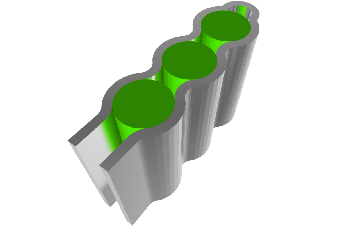
An example use case of a liquid-cooled battery pack is used here to demonstrate the application of PreonLab-TAITherm coupling. Battery cooling is an important thermal aspect in the emerging electric vehicle market. Figure 2 is a representation of a general battery pack that is cooled by a coolant flowing at a certain flow rate through a serpentine ribbon-shaped cooling tube. Each battery emits heat at a specific rate and is set to cool with the coolant interaction on the sides and with air cooling on the top surfaces.

As discussed above, simulations run in PreonLab and TAITherm one after the other utilizing the results from each other. The results from PreonLab are mapped as convective boundary conditions on the sides of the batteries in TAITherm. Other boundary conditions in TAITherm include the air cooling on the top surface, applied as a constant convective boundary condition and the heat generated within each of the battery cells. PreonLab maps the resulting temperature distribution of the battery surface from TAITherm and uses it as the temperature boundary condition to simulate the thermal interaction of the fluid flowing through the coolant tube.

Figure 3 shows the final steady-state temperature distribution of the surface of the battery. The figure shows the side where the coolant enters the coolant pipe (as indicated by the blue arrow). As can be seen, the temperature of the battery surfaces in contact with the coolant increases in the coolant flow direction, as the coolant heats up, reducing the heat absorption rate in the flow direction. Figure 4 shows the distribution of temperature within the coolant inside the coolant pipe.