This is just a selection of new features and improvements. Check out the changelog to learn about all changes. And enjoy our PreonLab 5.1 Release Event to learn more about what‘s going on in the PreonLab ecosystem.
Make sure to follow us on LinkedIn so that you don’t miss new videos, case studies and updates!
PRESENTER: Markus Ihmsen, Jens Cornelis, Jennifer Weiche,
Jan Viher
LANGUAGE: English
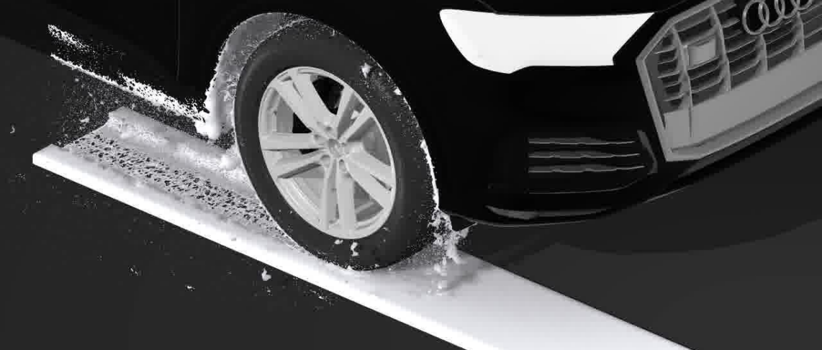
The snow solver is a distinguishing feature of PreonLab. Every version since PreonLab 4.0 has continuously improved the snow solver but PreonLab 5.1 has the biggest direct effect: The implicit solver now converges much faster to a qualitatively equivalent solution. As a result computing times for scenes with chunks of snow are down by an astonishing factor of five. Simulating one physical second in the example for instance took us 8 hours whereas now it only takes an 1 hour and 40 minutes. So if you don’t like waiting, consider updating to PreonLab 5.1 as soon as possible!
The capabilites of the PreonLab snow solver have been presented at the NAFEMS world congress 2021: “CFD Simulation of a Vehicle Driving in Snow” by D. Bäder (Audi AG, DEU) and A. Oliva, P. Kolar (AVL, DEU).
With new boundary conditions, scenes can now be set up and initialized in more detail than ever before. Many quantities that could only be provided as constant values can now be initialized on a per-particle level with PreonLab 5.1.
Area sources and volume sources can now assign individual temperatures to every newly generated particle based on a connected point cloud resource. In a similar manner, it is now also possible to map heat flux profiles onto solid surfaces as thermal boundary conditions. In case of the area source, you can also use the point cloud resource to map initial speeds to the releasing particles. We also added a predefined pipeflow velocity profile for convenience.
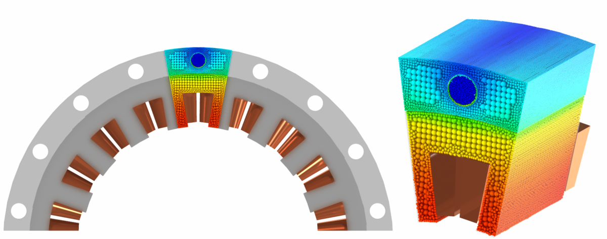
In this e-motor cooling example, the conjugate heat transfer is computed between fluid and engine parts. The heat transfer within the latter is performed using the Solid Volume Solver which supports adaptive resolution with 5.1. An initial guess of the temperature distribution within the solid parts was derived from an imported point cloud for faster convergence.
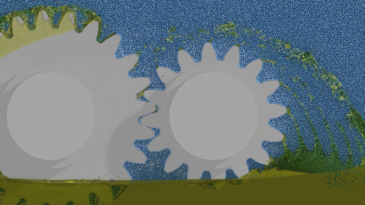
For many applications, single phase simulations are the best option to achieve good results quickly. In these cases, the contribution of other phases (typically air) is often modelled implicitly, for instance using PreonLab’s drag force object. However sometimes, the contribution of other phases is crucial and must be simulated explicitly to achieve meaningful results. With PreonLab 5.1, we have optimized multiphase to deliver better results for both low- and high-density contrasts. The quality of the simulation is improved using the new Continuum Surface Stress model which captures surface tension effects between the phases more accurately. To improve efficiency, we added the option to use different particle sizes for different phases. Additionally, it is also possible to use adaptive resolution for each phase. Last but not least we have developed best practices and workflows for some of the most common applications such as gearbox simulations.
In this example, oil and air (the blue particles) are simulated to compute accurate torque losses. Air particles are clipped using a plane so that oil is visible.
Adaptive resolution refines or coarsens particles on the fly as they enter or leave regions of interest. Since PreonLab 5.0, you can use three resolution levels to concentrate the computational power on the region where accuracy counts while saving performance in less prominent regions of the simulation domain.
PreonLab 5.1 introduces several changes that make adaptive resolution even better. Firstly, overall performance has been improved by up to 20%. Secondly, it is now possible to refine particles in proximity to selected geometries in the scene. In many cases, this allows to refine more precisely only where it matters, which can greatly improve overall performance. Thirdly, adaptive resolution now supports multiphase simulations, pathlines, periodic boundary conditions and the solid volume solver. This means that more applications can now be accelerated with adaptive resolution.
In this e-coating example, the new proximity refinement is used to accelerate the simulation. Only the fluid close to the car surface is simulated in high resolution.
Check out the changelog for a full list of changes. To learn more about the new features, have a look at the updated manual. We hope you will enjoy working with PreonLab 5.1 and as always, we would appreciate your feedback.