PreonLab

Planar Poiseuille Flow (2-D)

Validation objectives

The objective of this work is to test the capabilities of PreonLab in capturing the behavior of hydrodynamically fully developed 2-D internal flow between parallel plates (known as planar Poiseuille flow) for different Reynolds numbers within the laminar flow regime. Results are compared to the analytical solutions.

 Problem description

The problem consists of a Newtonian fluid with density ρ and viscosity µ between two parallel stationary plates (no-slip condition) which are infinitely long in the direction perpendicular to the x-y plane making it possible to assume the flow to be 2-dimensional.  Fluid is introduced with a uniform velocity of U_in in the positive x-direction at the inlet, see Fig. 1. The distance between the plates is 2h. In such flows, the region from the inlet to the point at which the boundary layers merge at the centerline is called the hydrodynamic entrance region. In this region, the flow is called hydrodynamically developing since the velocity profile develops there. The domain beyond the entrance region in which the velocity profile is fully developed and remains unchanged is called the hydrodynamically fully developed region, see Fig. 2. In the current study, the plates are long enough in the flow direction to include the hydrodynamically fully developed region.

The horizontal velocity profile u within the hydrodynamically fully developed region can be computed as:

where y is the distance from the centerline and h the distance between either of the plates from the centerline, see Fig. 1.

The shear stress at the wall τ_w is:

With u being the horizontal velocity and v the vertical velocity of the fluid.

Since from the continuity equation v = 0, one can write:

Therefore, in the hydrodynamically fully developed region:

Moreover, the pressure drop within this region can also be calculated as follows:

Benchmark quantities and target values
The following quantitative comparisons inside the fully developed region are performed:

1. Comparison of the velocity profiles within the hydrodynamically fully developed region at vertical planes with analytical solutions
2. Comparison of the pressure drop at mid-plane with analytical solutions
3. Comparison of the wall shear with analytical solutions

Test points

1. Reynolds number 10: h = 0.05 m, U_in = 0.034 m/s, ρ = 910 kg/m³, µ = 0.3094 Pa·s
   a. spacing 2mm
   b. spacing 1mm
2. Reynolds number 100: h = 0.05 m, U_in = 0.34 m/s, ρ = 910 kg/m³, µ = 0.3094 Pa·s
   a. spacing 2mm
   b. spacing 1mm
3. Reynolds number 1,000: h = 0.05 m, U_in = 3.4 m/s, ρ = 910 kg/m³, µ = 0.3094 Pa·s
   a. spacing 2mm
   b. spacing 1mm
4. Reynolds number 10: h = 0.05 m, U_in = 1 m/s, ρ = 100 kg/m³, µ = 1 Pa·s
   a. spacing 1mm
5. Reynolds number 100: h = 0.05 m, U_in = 1 m/s, ρ = 100 kg/m³, µ = 0.1 Pa·s
   a. spacing 1mm
6. Reynolds number 1,000: h = 0.05 m, U_in = 1 m/s, ρ = 100 kg/m³, µ = 0.01 Pa·s
   a. spacing 1mm

In test points 1 to 3, the inlet velocity is the variable to sweep Reynolds numbers. Moreover, in these test points, the resolution of the fluid, i.e., the particle spacing is varied in order to test resolution independency of the results.

Test points 4 to 6 are designed to evaluate parameter independence. Therefore, the density, inlet velocity and viscosity are different compared to test points 1 to 3. In test points 4 to 6, the viscosity value is the variable to sweep Reynolds numbers 10, 100 and 1,000. An example of the simulation results (test point 1) is shown in Fig. 3.

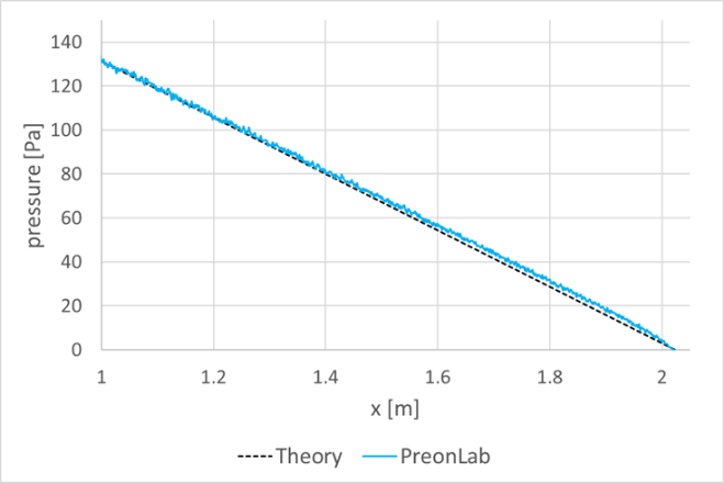
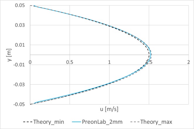
Discussion: The Lagrangian Preon solver discretizes the fluid volume and solves the low-compressible Navier-Stokes equations in an implicit and transient manner. It should be noted that this dynamic system poses some numerical challenges with respect to perfectly constant boundary conditions, particularly when generating a constant mass flow rate with a constant velocity. In this case, there can be small deviations between the nominal mass flow rate given as input to the solver and the one generated by the source. For the transient simulation, this deviation fluctuates over time. Accordingly, simulation results are compared with the analytical results based on the effective mean velocity on the vertical line inside the fully developed region.

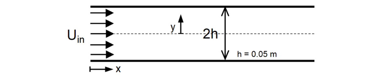
Test point 1 – Re = 10: U_in = 0.034 m/s, ρ = 910 kg/m³, µ = 0.3094 Pa·s

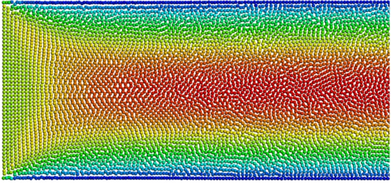
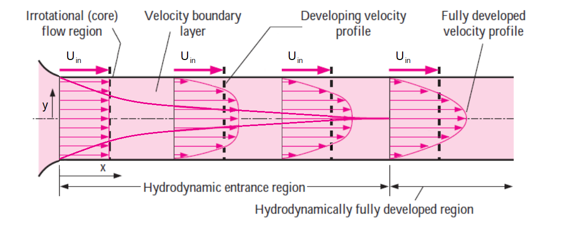
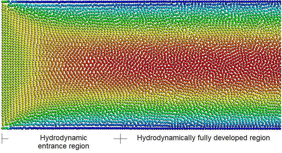
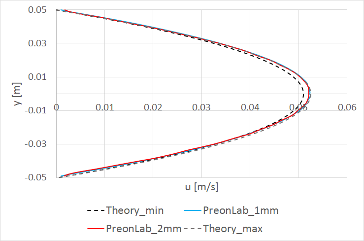
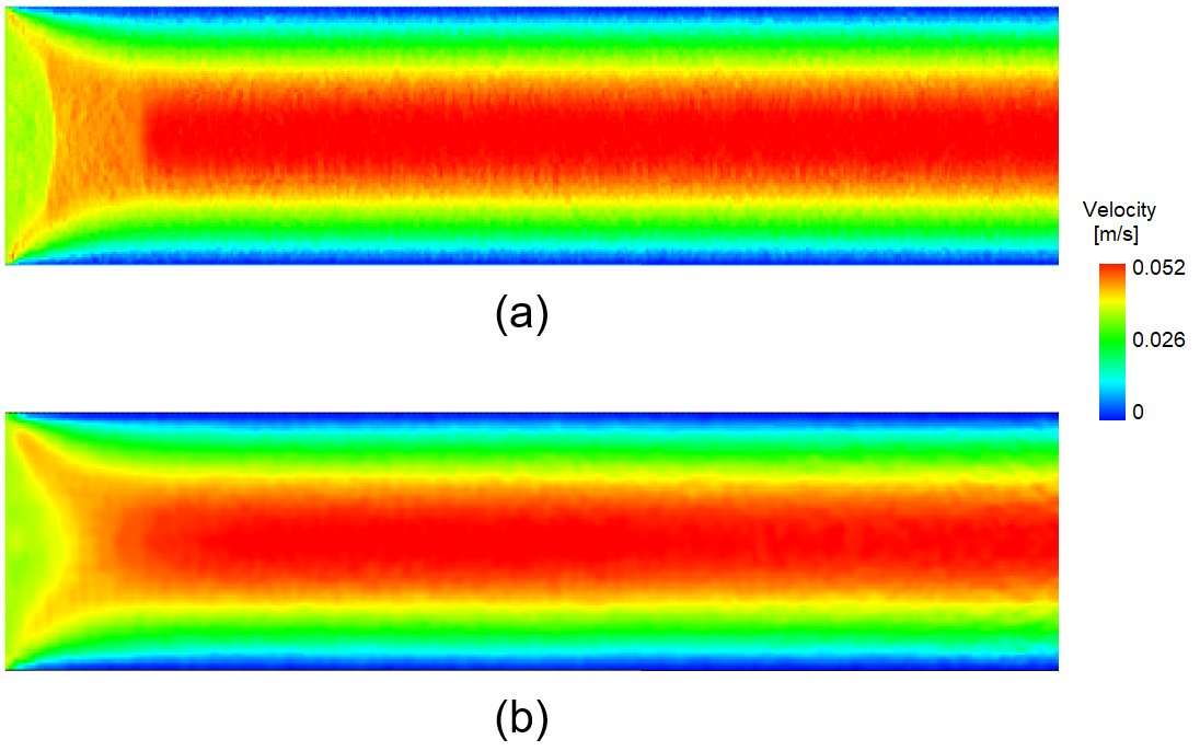
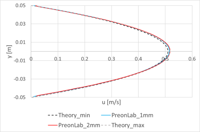
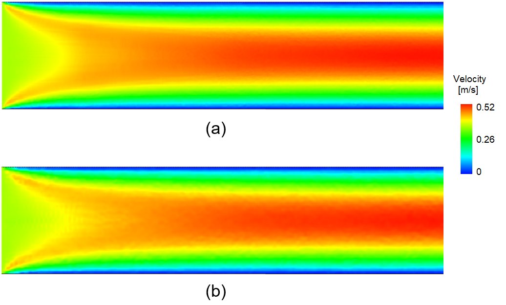
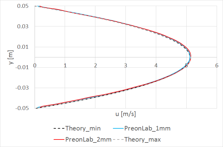
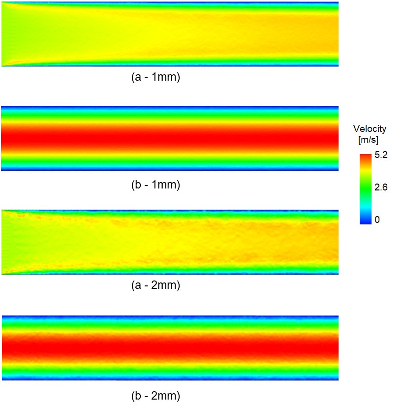
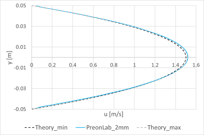
 At this test point, the horizontal velocity profile at the vertical line x = 1.4m located in the hydrodynamically fully developed region is compared to the analytical result. The mean velocity at this line fluctuates between 0.034 m/s and 0.035 m/s which equals a maximum error of ~3 percent with respect to the U_in boundary condition. As can be seen in Fig. 4, the velocity profiles for both simulations, using 1mm and 2mm spacings, are very much similar. In both cases, the results lie within the theoretical curves corresponding to the minimum and the maximum mean velocity values owing to the boundary conditions. Furthermore, the velocity fields are also compared for the two spacings in Fig. 5.

The pressure drop within the hydrodynamically fully developed region is known theoretically (see Section 1). A comparison between the time-averaged pressure on the centerline (between 50s and 60s) computed in PreonLab with the theoretical values is depicted in Fig. 6. Fluctuations in the simulation results are caused by the fact that simulations are performed in a transient manner which together with the density-invariant formulation and discretization of time imposes some challenges to keep the boundary conditions perfectly constant over time.

Test point 2 – Re = 100: U_in = 0.34 m/s, ρ = 910 kg/m³, µ = 0.3094 Pa·s

 A comparison of the horizontal velocity profile at the vertical line x = 1.39m to the analytical results is depicted in Fig. 7. The mean velocity at this line has a value between 0.34 m/s and 0.345 m/s representing a maximum corresponding error of less than 2 percent. Moreover, a comparison of the velocity fields for the two fluid spacings is illustrated in Fig. 8.

In Table 2, the time- and space-averaged wall shear on 0.1m of the wall length within the hydrodynamically fully developed region is compared to the theoretical value. The deviation is ~7% for the simulation with a particle spacing of 2mm and less than 1% for the simulation with 1mm spacing.

Test point 3 – Re = 1,000: U_in = 3.4 m/s, ρ = 910 kg/m³, µ = 0.3094 Pa·s

In Fig. 10, a comparison between the horizontal velocity profile at the vertical line x = 9m and the corresponding analytical results is depicted. The mean velocity value varies between
3.41 m/s and 3.43 m/s giving a maximum corresponding error of less than 1 percent. Furthermore, a comparison of the velocity fields for the two spacings in the hydrodynamic entry region as well as within the hydrodynamically fully developed region at t = 6s is illustrated in Fig. 11.

The time-averaged pressure on the centerline within the hydrodynamically fully developed region (between 5s and 6s) computed in PreonLab is compared to the theoretical values, see Fig. 12.

A comparison between the time- and space-averaged wall shear on 0.1m of the wall length within the hydrodynamically fully developed region with the theoretical value shows a good agreement. The deviation is ~4% for the simulation with a particle spacing of 2mm and ~2% for 1mm spacing, see Table 3.

Test point 4 – Re = 10: U_in = 1 m/s, ρ = 100 kg/m³, µ = 1 Pa·s

It can be seen from Fig. 13 that for test point 4 (Re = 10 but with a combination of parameters different from test point 1) the velocity profile at the vertical line x = 1.39m is in a good match with the analytical result.

Test point 5 – Re = 100: U_in = 1 m/s, ρ = 100 kg/m³, µ = 0.1 Pa·s

In test point 5, (Re = 100 with a combination of parameters alternative to test point 2) the velocity profile at x = 1.39m lies within the corresponding analytical range, see Fig. 14.

Test point 6 – Re = 1,000: U_in = 1 m/s, ρ = 100 kg/m³, µ = 0.01 Pa·s

As can be seen from Fig. 15, for test point 6 (alternative parameter set resulting in Re = 1,000) the velocity profile at x = 9m is in a good match with the analytical result.

In this study, PreonLab has successfully been validated against the analytical solution for a 2-D planar Poiseuille flow across Reynolds numbers ranging from 10 to 1,000 for different combinations of inlet velocity, viscosity and density. PreonLab is able to accurately reproduce time-averaged velocity profile, pressure drop and wall shear. Furthermore, it can be observed that varying the particle resolution from 1mm to 2mm only marginally affects the results. Thus, it can be concluded that PreonLab simulation has a high degree of resolution-independence for the aforementioned range of particle spacing in this validation benchmark.

[1] Cengel, Y. A. (2010). Fluid Mechanics: Fundamentals and Applications (SI Units). Tata McGraw Hill Education Private Limited.